
Volume 8, Issue 3 (10-2020)
Jorjani Biomed J 2020, 8(3): 4-18 |
Back to browse issues page


Download citation:
BibTeX | RIS | EndNote | Medlars | ProCite | Reference Manager | RefWorks
Send citation to:


BibTeX | RIS | EndNote | Medlars | ProCite | Reference Manager | RefWorks
Send citation to:
Karimi Darabi P, Tarokh M J. Type 2 Diabetes Prediction Using Machine Learning Algorithms. Jorjani Biomed J 2020; 8 (3) :4-18
URL: http://goums.ac.ir/jorjanijournal/article-1-738-en.html
URL: http://goums.ac.ir/jorjanijournal/article-1-738-en.html


1- Department of Industrial Engineering, K. N. Toosi University of Technology, Tehran, Iran , p_karimi@email.kntu.ac.ir
2- Department of Industrial Engineering, K. N. Toosi University of Technology, Tehran, Iran
2- Department of Industrial Engineering, K. N. Toosi University of Technology, Tehran, Iran
Full-Text [PDF 907 kb]
(2029 Downloads)
| Abstract (HTML) (4357 Views)
.png)
Fig 1. Support vector machine
.png) (2)
(2)

.png) (3)
(3)

Fig 3. A multilayer perceptron with two hidden layers (35)
.png)
Fig 4. Pre-processing flowchart
.png)
Fig 5. The attribute's correlation with the outcome
.png)
Fig 6. Statistical analysis for ML models
.png)
Fig 7. Receiver Operating Characteristic Curve (ROC) Metric
Conclusion
In this research, by applying eight learning machine algorithms, different models for diagnosis of diabetes were made. They were analyzed and compared with each other by using various valuation parameters. The result of the test shows that the gradient boosting model is the best model with an accuracy of 95.50% in the dataset of the Chinese population.
So far, machine learning methods have not been used to predict diabetes in the studied data set. This study could pave the way for others to research this data set. The basis of this study is to do more research and develop models such as other machine learning algorithm.
Full-Text: (1264 Views)
Introduction
According to the world health organization, diabetes is a chronic disease. This disease is due to either the pancreas not producing enough insulin or the body not responding properly to the insulin produced.
Diabetes has a serious global economic impact. In 2012, this disease with 1.5 million deaths, made the 8th leading cause of death. Based on statistics of 2017, nearly 425 million people had diabetes, about 2-5 million people die every year from diabetes disease. By 2045, it will reach 629 million (1).
This epidemic disease tends to grow. It was estimated that approximately 642 million people will have diabetes by 2040. However, the number of studies estimated that the annual cost of the disease from US$673 billion in 2015 reaches US$827 billion in 2016, which currently exceed the 2030 prediction (2).
Moreover, the economic burden of diabetes in China has risen over time. In 2015, the total annual expenditure was between US$51.1 and US$88.4 billion (3).
Type 1 diabetes is also called “insulin-dependent diabetes”. Type 1 diabetes results from the body’s inability to produce insulin. Therefore, the injection of insulin is essential for the patient. Type 2 diabetes occurs when the body’s cells do not react to insulin properly. This type of diabetes appears most often in middle-aged, and sometimes older people. Gestational diabetes is high blood sugar that develops during pregnancy in a woman who has not been diagnosed with diabetes before.
Today, the disease is also occurring in children. There are several causes of diabetes, including allergy, genetics, body weight, diet, physical activity, and, lifestyle (4).
Since diabetes is a multifactorial disease, it is diagnosis is complicated. Therefore, for accurate diagnosis, the physician should examine the test results of a patient, compare the test results with those of patients under the same condition, and analyze previous decisions. To care for a person, doctors are well prepared to identify people at risk for type 2 diabetes.
However, as we try to screen thousands of patients at high risk, the challenges that physicians face become apparent (26). and Analysis of the factors influencing the diagnosis may be influenced by human error. Because it is subject to the physician’s interpretation.
A Blood test is not discriminatory enough, and it is not enough for an accurate diagnosis of diabetes. Because among different characteristics of people it may be interpreted differently (4). Therefore, apart from laboratory information, lifestyle, physical condition, and family history of patients should be examined.
Despite human error probability, different types of machine learning algorithms, analytical and statistical methods, that use the previous and current data for finding information and predicting future events, can be used for solving this problem.
The artificial intelligence field is growing rapidly. Its functions in the field of diabetes are diagnosis and management of this chronic disease. The techniques of machine learning are used for making models of diabetes diagnosis and its side effects (5).
Results of empirical research articles, reflect the ability of analytical techniques to diagnose diabetes. Recent research shows that machine learning techniques can describe the characteristics of patients and identify patients at risk for type 2 diabetes (27,28). Machine Learning is one of the most important features of artificial intelligence that supports the development of computer systems with the ability to learn and improve from experiences, and the need to plan for every case (6).
The purpose of this study is to use learning machine algorithms for making models of type 2 diabetes diagnosis.
Related work
More than half of all adults worldwide are suffering from diabetes disease. Hence, early detection of the disease greatly improves patient quality of life. For the diagnosis of diabetes, a lot of researchers used learning machine methods and data analysis (7).
Many articles by using statistical analysis methods explored connections and samples between Chinese patients’ data (8-11).
Gao et al. in (8) used statistical analysis and multivariate Cox Regression algorithm to study the relationship between ALT and diabetes. They concluded that people between the age group 30-40 with elevated ALT are at a greater risk compared to those with low ALT.
Chen et al. in [9] by using statistical analysis and multivariate Cox Regression algorithm demonstrated that ratio TG /HDL-C was positively associated with the incidence of diabetes in the Chinese population.
Qin et al. in [3] by exploring ratio TG/HDL-C as an independent predictor of diabetes, found that TG/HDL-C is a powerful predictor in male patients compared to female patients.
Chen et al. in (10) investigated the relation of obesity and age with diabetes. Eventually, across all age groups, there was a linear association between BMI and diabetes. They verified that BMI and age are a strong predictor of diabetes.
Lin et al. in (11) designed a Nomogram based on the seven factors of diabetes in order to predict type 2 diabetes risk among people.
Diabetes prediction should be under control. Therefore, supervised learning algorithms have attracted a great deal of attention from researchers. By using machine learning, many diabetes research articles have been done on the Pima data set (12-15).
Wu et al. in (12) applied the Nearest Neighbor and Regression Logistic algorithms to make a diabetes prediction model with an accuracy of 95.42%.
Viloria et al. in (5) developed a diabetes predictive model by applying the Support Vector Machine algorithm. The algorithm was obtained with an accuracy of 99.2% with Colombian patients.
Devi et al. in (17) by employing a Support Vector Machine algorithm, managed to make a diabetes prediction model with an accuracy of 99.4%.
Many researchers also by analyzing different types of machine learning algorithms, assess and compare their performance on a particular data set, and, ultimately with particular evaluation methodologies, introduce the most appropriate predictive model for diabetes (18, 19).
Materials and Methods
Brief description of Machine Learning Classification Techniques
Logistic Regression
Logistic Regression (LR) is a sort of supervised learning which estimates the connection between a binary dependent variable and at least one independent variable by evaluating probabilities with the help of sigmoid function. In contrary to its name, LR is not used for regression problems rather is a type of machine learning classification problem where the dependent variable is dichotomous (0/1, -1/1, true/false) and independent variable can binominal, ordinal, interval or ratio-level. The sigmoid/Logistic function is given as:
.png) (1)
(1)
where, y is the output which is the result of weighted sum of input variables x. If the output is more than 0.5, the output is 1 else the output is 0 (19).
K-Nearest Neighbor
K-Nearest Neighbor (KNN) method can be used for both classification and regression problems (19). However, it is more widely used in classification problems in the industry. KNN is a simple algorithm that stores all available cases and classifies new cases by a majority vote of its k neighbors. The case is assigned to the class is most common amongst its K nearest neighbors measured by a distance function. These distance functions can be Euclidean, Manhattan, Minkowski, and Hamming distance.
The first three functions are used for continuous function and the fourth one (Hamming) for categorical variables. If K = 1, then the case is simply assigned to the class of its nearest neighbor. At times, choosing K turns out to be a challenge while performing KNN modeling. Its major advantage is the simplicity of translation and low computation time.
Support Vector Machine
Support Vector Machine (SVM) is a supervised classifier in machine learning algorithms that can be used both for regression and classification. It is majorly applied in solving classification problems. The goal of SVM is to classify data points by an appropriate hyperplane in a multidimensional space. A hyperplane is a decision boundary to classify data points. The hyperplane classifies the data points with the maximum margin between the classes and the hyperplane (19).
In this algorithm, we plot each data item as a point in n-dimensional space (where n is the number of features you have) with the value of each feature being the value of a particular coordinate. For example, if we only had two features like Height and Hair length of an individual, we’d first plot these two variables in two-dimensional space where each point has two coordinates (these coordinates are known as Support Vectors) In fig 1, the line which splits the data into two differently classified groups is the black line since the two closest points are the farthest apart from the line. This line is our classifier. Then, depending on where the testing data lands on either side of the line, that’s what class we can classify the new data as (25).
According to the world health organization, diabetes is a chronic disease. This disease is due to either the pancreas not producing enough insulin or the body not responding properly to the insulin produced.
Diabetes has a serious global economic impact. In 2012, this disease with 1.5 million deaths, made the 8th leading cause of death. Based on statistics of 2017, nearly 425 million people had diabetes, about 2-5 million people die every year from diabetes disease. By 2045, it will reach 629 million (1).
This epidemic disease tends to grow. It was estimated that approximately 642 million people will have diabetes by 2040. However, the number of studies estimated that the annual cost of the disease from US$673 billion in 2015 reaches US$827 billion in 2016, which currently exceed the 2030 prediction (2).
Moreover, the economic burden of diabetes in China has risen over time. In 2015, the total annual expenditure was between US$51.1 and US$88.4 billion (3).
Type 1 diabetes is also called “insulin-dependent diabetes”. Type 1 diabetes results from the body’s inability to produce insulin. Therefore, the injection of insulin is essential for the patient. Type 2 diabetes occurs when the body’s cells do not react to insulin properly. This type of diabetes appears most often in middle-aged, and sometimes older people. Gestational diabetes is high blood sugar that develops during pregnancy in a woman who has not been diagnosed with diabetes before.
Today, the disease is also occurring in children. There are several causes of diabetes, including allergy, genetics, body weight, diet, physical activity, and, lifestyle (4).
Since diabetes is a multifactorial disease, it is diagnosis is complicated. Therefore, for accurate diagnosis, the physician should examine the test results of a patient, compare the test results with those of patients under the same condition, and analyze previous decisions. To care for a person, doctors are well prepared to identify people at risk for type 2 diabetes.
However, as we try to screen thousands of patients at high risk, the challenges that physicians face become apparent (26). and Analysis of the factors influencing the diagnosis may be influenced by human error. Because it is subject to the physician’s interpretation.
A Blood test is not discriminatory enough, and it is not enough for an accurate diagnosis of diabetes. Because among different characteristics of people it may be interpreted differently (4). Therefore, apart from laboratory information, lifestyle, physical condition, and family history of patients should be examined.
Despite human error probability, different types of machine learning algorithms, analytical and statistical methods, that use the previous and current data for finding information and predicting future events, can be used for solving this problem.
The artificial intelligence field is growing rapidly. Its functions in the field of diabetes are diagnosis and management of this chronic disease. The techniques of machine learning are used for making models of diabetes diagnosis and its side effects (5).
Results of empirical research articles, reflect the ability of analytical techniques to diagnose diabetes. Recent research shows that machine learning techniques can describe the characteristics of patients and identify patients at risk for type 2 diabetes (27,28). Machine Learning is one of the most important features of artificial intelligence that supports the development of computer systems with the ability to learn and improve from experiences, and the need to plan for every case (6).
The purpose of this study is to use learning machine algorithms for making models of type 2 diabetes diagnosis.
Related work
More than half of all adults worldwide are suffering from diabetes disease. Hence, early detection of the disease greatly improves patient quality of life. For the diagnosis of diabetes, a lot of researchers used learning machine methods and data analysis (7).
Many articles by using statistical analysis methods explored connections and samples between Chinese patients’ data (8-11).
Gao et al. in (8) used statistical analysis and multivariate Cox Regression algorithm to study the relationship between ALT and diabetes. They concluded that people between the age group 30-40 with elevated ALT are at a greater risk compared to those with low ALT.
Chen et al. in [9] by using statistical analysis and multivariate Cox Regression algorithm demonstrated that ratio TG /HDL-C was positively associated with the incidence of diabetes in the Chinese population.
Qin et al. in [3] by exploring ratio TG/HDL-C as an independent predictor of diabetes, found that TG/HDL-C is a powerful predictor in male patients compared to female patients.
Chen et al. in (10) investigated the relation of obesity and age with diabetes. Eventually, across all age groups, there was a linear association between BMI and diabetes. They verified that BMI and age are a strong predictor of diabetes.
Lin et al. in (11) designed a Nomogram based on the seven factors of diabetes in order to predict type 2 diabetes risk among people.
Diabetes prediction should be under control. Therefore, supervised learning algorithms have attracted a great deal of attention from researchers. By using machine learning, many diabetes research articles have been done on the Pima data set (12-15).
Wu et al. in (12) applied the Nearest Neighbor and Regression Logistic algorithms to make a diabetes prediction model with an accuracy of 95.42%.
Viloria et al. in (5) developed a diabetes predictive model by applying the Support Vector Machine algorithm. The algorithm was obtained with an accuracy of 99.2% with Colombian patients.
Devi et al. in (17) by employing a Support Vector Machine algorithm, managed to make a diabetes prediction model with an accuracy of 99.4%.
Many researchers also by analyzing different types of machine learning algorithms, assess and compare their performance on a particular data set, and, ultimately with particular evaluation methodologies, introduce the most appropriate predictive model for diabetes (18, 19).
Materials and Methods
Brief description of Machine Learning Classification Techniques
Logistic Regression
Logistic Regression (LR) is a sort of supervised learning which estimates the connection between a binary dependent variable and at least one independent variable by evaluating probabilities with the help of sigmoid function. In contrary to its name, LR is not used for regression problems rather is a type of machine learning classification problem where the dependent variable is dichotomous (0/1, -1/1, true/false) and independent variable can binominal, ordinal, interval or ratio-level. The sigmoid/Logistic function is given as:
(1)where, y is the output which is the result of weighted sum of input variables x. If the output is more than 0.5, the output is 1 else the output is 0 (19).
K-Nearest Neighbor
K-Nearest Neighbor (KNN) method can be used for both classification and regression problems (19). However, it is more widely used in classification problems in the industry. KNN is a simple algorithm that stores all available cases and classifies new cases by a majority vote of its k neighbors. The case is assigned to the class is most common amongst its K nearest neighbors measured by a distance function. These distance functions can be Euclidean, Manhattan, Minkowski, and Hamming distance.
The first three functions are used for continuous function and the fourth one (Hamming) for categorical variables. If K = 1, then the case is simply assigned to the class of its nearest neighbor. At times, choosing K turns out to be a challenge while performing KNN modeling. Its major advantage is the simplicity of translation and low computation time.
Support Vector Machine
Support Vector Machine (SVM) is a supervised classifier in machine learning algorithms that can be used both for regression and classification. It is majorly applied in solving classification problems. The goal of SVM is to classify data points by an appropriate hyperplane in a multidimensional space. A hyperplane is a decision boundary to classify data points. The hyperplane classifies the data points with the maximum margin between the classes and the hyperplane (19).
In this algorithm, we plot each data item as a point in n-dimensional space (where n is the number of features you have) with the value of each feature being the value of a particular coordinate. For example, if we only had two features like Height and Hair length of an individual, we’d first plot these two variables in two-dimensional space where each point has two coordinates (these coordinates are known as Support Vectors) In fig 1, the line which splits the data into two differently classified groups is the black line since the two closest points are the farthest apart from the line. This line is our classifier. Then, depending on where the testing data lands on either side of the line, that’s what class we can classify the new data as (25).
Fig 1. Support vector machine
Naive Bayesian
The naive Bayesian (NB) method is a classification technique based on Bayes’ theorem with an assumption of independence between predictors. Even with its simplicity, it outperforms other classifiers, hence, it is one of the best classifier (30,19). In simple terms, a Naive Bayes classifier assumes that the presence of a particular feature in a class is unrelated to the presence of any other feature. The naive Bayesian model is easy to build and particularly useful for very large data sets. Along with simplicity, Naive Bayes is known to outperform even highly sophisticated classification methods.
Bayes theorem provides a way of calculating posterior probability P(c|x) from P(c), P(x), and P(x|c). Look at the equation below:
(2)(3)Here,
- P(c|x) is the posterior probability of class (target) given predictor (attribute).
- P(c) is the prior probability of class.
- P(x|c) is the likelihood which is the probability of predictor given class.
- P(x) is the prior probability of predictor.
Decision Tree
A Decision Tree (DT) is working on the principle of decision making. It can be described in the form of a tree and provides high accuracy and stability. Fig 2 illustrates a decision tree (19). It is a type of supervised learning algorithm that is mostly used for classification problems. Surprisingly, it works for both categorical and continuous dependent variables. In this algorithm, we split the population into two or more homogeneous sets. This is done based on the most significant attributes/ independent variables to make as distinct groups as possible.

Fig 2. The Decision Tree
Random Forest
The Random Forest (RF) classifier creates multiple decision trees from a randomly selected subset of the training dataset. Then it aggregates the votes from different decision trees to decide the final class of test objects (19). To classify a new object based on attributes, each tree gives a classification and we say the tree “votes” for that class. The forest chooses the classification having the most votes (over all the trees in the forest). Each tree is planted & grown as follows:
1. If the number of cases in the training set is N, then a sample of N cases is taken at random but with replacement. This sample will be the training set for growing the tree.
2. If there are M input variables, a number m< 3. Each tree is grown to the largest extent possible. There is no pruning.
Neural Network
Neural networks, or more precisely artificial neural networks, are a branch of artificial intelligence. Multilayer perceptrons form one type of neural network. Unlike other statistical techniques the multilayer perceptron makes no prior assumptions concerning the data distribution.
It can model highly non-linear functions and can be trained to accurately generalise when presented with new, unseen data. These features of the multilayer perceptron make it an attractive alternative to developing numerical models, and also when choosing between statistical approaches.
The multilayer perceptron consists of a system of simple interconnected neurons, or nodes, as illustrated in Fig. 3, which is a model representing a nonlinear mapping between an input vector and an output vector. The nodes are connected by weights and output signals which are a function of the sum of the inputs to the node modified by a simple nonlinear transfer, or activation, function. It is the superposition of many simple nonlinear transfer functions that enables the multilayer perceptron to approximate extremely non-linear functions (31).
- P(c|x) is the posterior probability of class (target) given predictor (attribute).
- P(c) is the prior probability of class.
- P(x|c) is the likelihood which is the probability of predictor given class.
- P(x) is the prior probability of predictor.
Decision Tree
A Decision Tree (DT) is working on the principle of decision making. It can be described in the form of a tree and provides high accuracy and stability. Fig 2 illustrates a decision tree (19). It is a type of supervised learning algorithm that is mostly used for classification problems. Surprisingly, it works for both categorical and continuous dependent variables. In this algorithm, we split the population into two or more homogeneous sets. This is done based on the most significant attributes/ independent variables to make as distinct groups as possible.
Fig 2. The Decision Tree
Random Forest
The Random Forest (RF) classifier creates multiple decision trees from a randomly selected subset of the training dataset. Then it aggregates the votes from different decision trees to decide the final class of test objects (19). To classify a new object based on attributes, each tree gives a classification and we say the tree “votes” for that class. The forest chooses the classification having the most votes (over all the trees in the forest). Each tree is planted & grown as follows:
1. If the number of cases in the training set is N, then a sample of N cases is taken at random but with replacement. This sample will be the training set for growing the tree.
2. If there are M input variables, a number m<
Neural Network
Neural networks, or more precisely artificial neural networks, are a branch of artificial intelligence. Multilayer perceptrons form one type of neural network. Unlike other statistical techniques the multilayer perceptron makes no prior assumptions concerning the data distribution.
It can model highly non-linear functions and can be trained to accurately generalise when presented with new, unseen data. These features of the multilayer perceptron make it an attractive alternative to developing numerical models, and also when choosing between statistical approaches.
The multilayer perceptron consists of a system of simple interconnected neurons, or nodes, as illustrated in Fig. 3, which is a model representing a nonlinear mapping between an input vector and an output vector. The nodes are connected by weights and output signals which are a function of the sum of the inputs to the node modified by a simple nonlinear transfer, or activation, function. It is the superposition of many simple nonlinear transfer functions that enables the multilayer perceptron to approximate extremely non-linear functions (31).
Fig 3. A multilayer perceptron with two hidden layers (35)
Gradient Boosting
Gradient boosting methods construct the solution in a stage-wise fashion and solve the overfitting problem by optimizing the loss functions. For example, assume that you have a custom base-learner h(x, θ) (such as decision tree), and a loss function 𝜓(y, f(x)); it is challenging to estimate the parameters directly, and thus, an iterative model is suggested such that at each iteration. The model will be updated and a new base-learner function h (x, θt) is where the increment is guided by:
 f(x)=ft-1(x) (4)
This allows the substitution of the hard optimization problem with the usual least-squares optimization problem:
.png) 2 (5)
2 (5)
Gradient boosting methods construct the solution in a stage-wise fashion and solve the overfitting problem by optimizing the loss functions. For example, assume that you have a custom base-learner h(x, θ) (such as decision tree), and a loss function 𝜓(y, f(x)); it is challenging to estimate the parameters directly, and thus, an iterative model is suggested such that at each iteration. The model will be updated and a new base-learner function h (x, θt) is where the increment is guided by:
f(x)=ft-1(x) (4) This allows the substitution of the hard optimization problem with the usual least-squares optimization problem:
2 (5)| Algorithm1 gradient boost |
| 1. Let ƒ0 be a constant 2. For i = 1 to M a. Compute gi(x) using eq() b. Train the function h (x, θi) c. Find 𝜌i using eq() d. Update the function 𝑓i = 𝑓i-1 + 𝜌i ℎ (𝑥, 𝜃i) 3. End |
The algorithm starts with a single leaf, and then the learning rate is optimized for each node and each record (22-24,29).
performance evaluation metrics
One of the most important steps after designing and building a model is evaluating its performance. In this section, the performance of the proposed algorithms, concerning different performance parameters such as Accuracy, Confusion Matrix, Sensitivity, Specificity, Recall, F1_Score, ROC, MSE and RMSE.
Confusion matrix
The information about actual and predicted classification system is hold by the Confusion Matrix. It demonstrates the accuracy of the solution to a classification problem. Table 2 shows the Confusion Matrix for a two class classifier. The entries in the Confusion Matrix have the following meaning in the context of our study. TP is the number of correct predictions that an instance is positive. FN is the number of incorrect predictions that an instance is negative. FP is the number of incorrect predictions that an instance is positive and is the number of correct predictions that an TP instance is negative (12).
Table 1. The Confusion Matrix for a two class classifier
| Prediction | |||
| Positive | Negative | ||
| Actual | Positive Negative |
TP FP |
FN TN |
Classification Accuracy
It is one of the most popular metrics in classifier evaluation. It is the proportion of the number of positive tuples and negative tuples obtained by the classification algorithms in the total number of occurrences [17], as given by
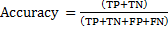 (6)
(6)
Sensitivity
Proportion of positive cases that are well detected by the test. In other words, the sensitivity measures how the test is effective when used on positive individuals. The mathematical definition is given by:
 (7)
(7)
Specificity
Proportion of negative cases that are well detected by the test. In other words, specificity measures how the test is effective when used on negative individuals. The mathematical definition is given by:
 (8)
(8)
Precision
Precision looks at the ratio of correct positive observations. The formula is,
 (9)
(9)
Recall
Recall is also known as sensitivity or true positive rate. It’s the ratio of correctly predicted positive events.
.png) (10)
(10)
F1_ Score
F1-Score is the choral mean of precision and recall, as given byEq. (11). F1-Score takes on values from 0 to 1. The higher value of F1-Score, the better the classification algorithm is (17).
.png) (11)
(11)
ROC
It is another common metric for evaluating the classifiers. It equals to the probability that a classifier will rank a randomly chosen positive instance higher than a randomly chosen negative one. It takes on values from 0 to 1. The better classification is based on the higher the value of ROC (17).
Mean Squared Error
MSE tells you how close a regression line is to a set of points. It does this by taking the distances from the points to the regression line (these distances are the “errors”) and squaring them. The squaring is necessary to remove any negative signs. It also gives more weight to larger differences. It’s called the mean squared error as you’re finding the average of a set of errors.
 (12)
(12)
Root mean square error
RMSE is a quadratic scoring rule that also measures the average magnitude of the error. It’s the square root of the average of squared differences between prediction and actual observation.
 (13)
(13)
Data Description
Study population
The clinical data of the population we studied were obtained from the ‘Dryad Digital Repository[1]’ (20). This website makes the raw data of published papers freely reusable for secondary analysis. According to the Dryad Terms of Service, we cited the Dryad data package in the present study (20). Chen et al. conducted a retrospective cohort study of adult individuals across 11 cities in China (21). 211,833 persons free of diabetes at baseline and with at least 2 visits between 2010 and 2016 were recruited.
Data definition
We extracted variables from the database as follows: age, gender, body mass index (BMI), systolic blood pressure (SBP), diastolic blood pressure (DBP), smoking and drinking status, family history of diabetes, alanine aminotransferase (ALT), fasting plasma glucose (FPG), total cholesterol (TC), low density lipoprotein (LDL), high density lipoprotein cholesterol (HDL-C), triglyceride (TG), year of follow up, and finally diagnosed of diabetes. For more details, you can read: [21]
Data pre-processing
In this study, data from e-health records were used in 32 health care centers in 11 provinces in China. The data pre-processing flowchart (fig 4) can be used as a reference when reading this paragraph. After manually removing the variables of height, follow-up, and censorship of the disease, the number of variables was reduced to 20 Then all variables with missing values above 50% were deleted. Similarly, this filtering was done at the level of individual records. The majority of registered cases complied with the missing value rule above 50%. An important issue in pre-processing was the imbalance of the data. Out of 32,312 cases, only 1304 were diabetic patients. Therefore, the sampling of the data set should be done to balance the data set. Finally, the prepared data set includes 5000 records with 19 variables. Examples and variables of our data set, along with some statistical information are described in Table 2. Also, a visual representation of the data set variables and the correlations between them can be seen in Fig 5.
It is one of the most popular metrics in classifier evaluation. It is the proportion of the number of positive tuples and negative tuples obtained by the classification algorithms in the total number of occurrences [17], as given by
(6)Sensitivity
Proportion of positive cases that are well detected by the test. In other words, the sensitivity measures how the test is effective when used on positive individuals. The mathematical definition is given by:
(7)Specificity
Proportion of negative cases that are well detected by the test. In other words, specificity measures how the test is effective when used on negative individuals. The mathematical definition is given by:
(8)Precision
Precision looks at the ratio of correct positive observations. The formula is,
(9)Recall
Recall is also known as sensitivity or true positive rate. It’s the ratio of correctly predicted positive events.
(10)F1_ Score
F1-Score is the choral mean of precision and recall, as given byEq. (11). F1-Score takes on values from 0 to 1. The higher value of F1-Score, the better the classification algorithm is (17).
(11)ROC
It is another common metric for evaluating the classifiers. It equals to the probability that a classifier will rank a randomly chosen positive instance higher than a randomly chosen negative one. It takes on values from 0 to 1. The better classification is based on the higher the value of ROC (17).
Mean Squared Error
MSE tells you how close a regression line is to a set of points. It does this by taking the distances from the points to the regression line (these distances are the “errors”) and squaring them. The squaring is necessary to remove any negative signs. It also gives more weight to larger differences. It’s called the mean squared error as you’re finding the average of a set of errors.
(12)Root mean square error
RMSE is a quadratic scoring rule that also measures the average magnitude of the error. It’s the square root of the average of squared differences between prediction and actual observation.
(13)Data Description
Study population
The clinical data of the population we studied were obtained from the ‘Dryad Digital Repository[1]’ (20). This website makes the raw data of published papers freely reusable for secondary analysis. According to the Dryad Terms of Service, we cited the Dryad data package in the present study (20). Chen et al. conducted a retrospective cohort study of adult individuals across 11 cities in China (21). 211,833 persons free of diabetes at baseline and with at least 2 visits between 2010 and 2016 were recruited.
Data definition
We extracted variables from the database as follows: age, gender, body mass index (BMI), systolic blood pressure (SBP), diastolic blood pressure (DBP), smoking and drinking status, family history of diabetes, alanine aminotransferase (ALT), fasting plasma glucose (FPG), total cholesterol (TC), low density lipoprotein (LDL), high density lipoprotein cholesterol (HDL-C), triglyceride (TG), year of follow up, and finally diagnosed of diabetes. For more details, you can read: [21]
Data pre-processing
In this study, data from e-health records were used in 32 health care centers in 11 provinces in China. The data pre-processing flowchart (fig 4) can be used as a reference when reading this paragraph. After manually removing the variables of height, follow-up, and censorship of the disease, the number of variables was reduced to 20 Then all variables with missing values above 50% were deleted. Similarly, this filtering was done at the level of individual records. The majority of registered cases complied with the missing value rule above 50%. An important issue in pre-processing was the imbalance of the data. Out of 32,312 cases, only 1304 were diabetic patients. Therefore, the sampling of the data set should be done to balance the data set. Finally, the prepared data set includes 5000 records with 19 variables. Examples and variables of our data set, along with some statistical information are described in Table 2. Also, a visual representation of the data set variables and the correlations between them can be seen in Fig 5.
| Variables Name | Normal Interval | Mean, STD | Type |
| Age | 20-93 | 48.085057-14.686155 | N |
| Gender | Female or Male | 1.351615-0.477530 | N |
| Weight | 36-141 (kg) | 67.525920-12.443953 | N |
| BMI | 15.2-45.8 (kg/m2) | 24.123923-3.397294 | N |
| SBP | 77-200 (mmHg) | 123.219382-17.513858 | N |
| DBP | 44-134 (mmHg) | 76.360446-11.004056 | N |
| FPG | 1.78-6.99 (mmol/L) | 5.226368-0.781089 | N |
| FFPG | 3.2-29.7 (mmol/L) | 5.729084-1.424568 | N |
| Cholesterol | 2.12-11.65 (mmol/L) | 4.860753-0.925377 | N |
| Triglyceride | 0-32.64 (mmol/L) | 1.588476-1.260003 | N |
| HDL | 0-2.85 (mmol/L) | 1.666765-1.079377 | N |
| LDL | 0.55-6.75 (U/L) | 2.976220-0.892196 | N |
| ALT | 0.4-365.7 (mmol/L) | 26.754810-22.279922 | N |
| BUN | 1.38-17.73 (mmol/L) | 4.841088-1.251566 | N |
| CCR | 33.9-307 (mmol/L) | 71.557080-16.937394 | N |
| Smoking status | 1, current smoker 2, ever smoker 3, never smoker |
3.006123-1.199571 | N |
| Drinking status | 1, current drinker 2, ever drinker 3, never drinker |
3.209935-0.939842 | N |
| Family history | 0-1 | 0.061585-0.240428 | N |
| Diabetes | 0-1 | 0.302812-0.459528 | N |
Fig 4. Pre-processing flowchart
Fig 5. The attribute's correlation with the outcome
Model selection using k-fold cross validation
In our work, we have carried out parameter tuning, have trained models with optimal parameters, and made predictions using these models by implementing the k-fold cross-validation procedure.
In our work, we have carried out parameter tuning, have trained models with optimal parameters, and made predictions using these models by implementing the k-fold cross-validation procedure.
| Algorithm: proposed method for type 2 diabetes prediction |
| 1. begin 2. pre-processing of the dataset different statistical techniques 3. using k-fold cross validation technique for tuning parameters and best model selection 4. classification of diabetes and healthy people using GBM, LR, KNN, NB, DT, RF, SVM, NN classifiers 5. computes different performance evaluation metrics for model evaluation 6. selection best model for type 2 diabetes 7. end |
The cross-validation steps be summarized as follows:
Step 1. The available dataset is split into two parts, training and an independent test set. The training set is used for parameter tuning and test set for the final model evaluation step at the end i.e. at Step 5. In our work, 70% of the combined dataset is randomly selected from the available dataset to be used as the training set while the remaining 30% is used as the test set.
Step 2. In the second step, we specify the range of values for the different parameters that are to be tuned.
Step 3. In this step, for each parameter configuration, the k-fold cross-validation is applied to the training set. The best parameter configuration is identified. we utilized a grid search to identify the best set of parameters of the models generated from different methods. 10-fold stratified cross-validation (SCV) was utilized by us. Accuracy was used as the performance measure to evaluate the parameters.
Step 4. In this step, models of algorithms are constructed using the optimal parameters obtained in the previous step.
Step 5. In this step, the test data set mentioned in the first step is used to evaluate the models made in step 4. The model that has the best set of evaluation criteria in evaluations. Selected as the best model.
Step 6. Finally, after evaluating the models, after combining the training and test sets, the winning model can be fitted to all data. This model can be used for deployment.
Result and Discussion
Statistical analysis and model validation
In this section, the models are compared with each other to show their performance based on the dataset of China population. High accuracy means that the model predicts the accurate output. By considering accuracy, it could be possible to understand whether the model was trained well or not. Generally, how is its performance? Consequently, in analyzing the results of model accuracy, the gradient boosting model had shown the best performance. However, this criterion does not give detailed information about model performance. Therefore, there is a need for other criteria in order to analyze further.
To compare the machine learning methods, the diabetic dataset is used and tested by implementing LR, DT, RF, SVM, NB, GBM, KNN, and NN. The training Accuracy, test Accuracy, Sensitivity, Specificity, Precision, F1_Score, MSE, RMSE of performance metrics for ML models, are reported in Table 3 and fig 6. These metrics have been calculated using the test set.
| ROC | RMSE | MSE | F1 | Pr | SP | SE | Test Acc | Trainig Acc | Algorithm |
| 0.93 | 0.215 | 0.046 | 0.916 | 0.945 | 0.889 | 0.979 | 0.953 | 0.956 | LR |
| 0.94 | 0.215 | 0.046 | 0.917 | 0.933 | 0.9 | 0.973 | 0.953 | 0.954 | DT |
| 0.93 | 0.219 | 0.048 | 0.913 | 0.942 | 0.886 | 0.978 | 0.953 | 1 | RF |
| 0.93 | 0.213 | 0.045 | 0.916 | 0.964 | 0.873 | 0.986 | 0.954 | 0.956 | SVM |
| 0.92 | 0.252 | 0.063 | 0.889 | 0.889 | 0.889 | 0.955 | 0.936 | 0.946 | NB |
| 0.94 | 0.211 | 0.045 | 0.917 | 0.924 | 0.9 | 0.988 | 0.955 | 1 | GBM |
| 0.92 | 0.226 | 0.051 | 0.906 | 0.955 | 0.862 | 0.983 | 0.948 | 0.964 | KNN |
| 0.93 | 0.236 | 0.055 | 0.901 | 0.911 | 0.892 | 0.965 | 0.944 | 0.981 | NN |
Table 3. Statistical measures of different ML models
From the results presented in Table 3, it can be observed that out of the compared algorithms, NB performed the worst on the test set. The NB model possesses the lowest values for all metrics. This is in an agreement where NB performed the worst amongst the ML methods compared to them.
KNN and NN (1_layer perceptron) in our work, performs significantly better than NB. In the same way, LR and RF perform better than the NB, KNN, and NN classifiers and are fourth and Fifth best in terms of the values of metrics.
SVM performs better than the other classifiers and is Third best in terms of the values of the Precision and MSE. The values are 0.964 and 0.045 respectively. DT performs better than the other classifiers and is second best in terms of the values of the SP, F1, and ROC. The values are 0.900, 0.917 and 0.94 respectively.
Among them, GBM possessed the highest performance metrics with Train Acc, Test Acc, SE, SP, F1, MSE, and RMSE being 1, 0.955, 0.988, 0.900, 0.917, 0.045, and 0.211 respectively. Since GBM is scalable, has the potential to serve as a general-purpose algorithm to develop models for diabetes predictor using datasets.
Fig 6. Statistical analysis for ML models
In terms of area under the receiver operating characteristic curve (ROC) metric, GBM and DT outperformed other compared methods on datasets. GBM and DT maintained the best results with the ROC of 0.94, compared to other ML methods. (see Fig 7)
Fig 7. Receiver Operating Characteristic Curve (ROC) Metric
Conclusion
In this research, by applying eight learning machine algorithms, different models for diagnosis of diabetes were made. They were analyzed and compared with each other by using various valuation parameters. The result of the test shows that the gradient boosting model is the best model with an accuracy of 95.50% in the dataset of the Chinese population.
So far, machine learning methods have not been used to predict diabetes in the studied data set. This study could pave the way for others to research this data set. The basis of this study is to do more research and develop models such as other machine learning algorithm.
|
Type of Article: Original article |
Subject:
Bio-statistics
Received: 2020/07/15 | Accepted: 2020/08/5 | Published: 2020/10/1
Received: 2020/07/15 | Accepted: 2020/08/5 | Published: 2020/10/1
References
1. Carter, Jake A., et al. "Combining elemental analysis of toenails and machine learning techniques as a non-invasive diagnostic tool for the robust classification of type-2 diabetes." Expert Systems with Applications 115 (2019): 245-255. [view at publisher] [DOI] [Google Scholar]
2. Ogurtsova, Katherine, et al. "IDF Diabetes Atlas: Global estimates for the prevalence of diabetes for 2015 and 2040." Diabetes research and clinical practice 128 (2017): 40-50. [view at publisher] [DOI] [Google Scholar]
3. Qin, Hailun, et al. "Triglyceride to high‐density lipoprotein cholesterol ratio is associated with incident diabetes in men: A retrospective study of Chinese individuals." Journal of Diabetes Investigation 11.1 (2020): 192-198. [view at publisher] [DOI] [Google Scholar]
4. Mujumdar, Aishwarya, and V. Vaidehi. "Diabetes prediction using machine learning algorithms." Procedia Computer Science 165 (2019): 292-299. [view at publisher] [DOI] [Google Scholar]
5. Zhang, Liying, et al. "Machine learning for characterizing risk of type 2 diabetes mellitus in a rural Chinese population: The Henan Rural Cohort Study." Scientific reports 10.1 (2020): 1-10. [DOI] [Google Scholar]
6. Viloria, Amelec, et al. "Diabetes Diagnostic Prediction Using Vector Support Machines." Procedia Computer Science 170 (2020): 376-381. [view at publisher] [DOI] [Google Scholar]
7. Dinh, A., Miertschin, S., Young, A. & Mohanty, S. D. A data-driven approach to predicting diabetes and cardiovascular disease with machine learning. BMC Med. Inform. Decis. Mak. 19, 211 (2019). [view at publisher] [DOI] [Google Scholar]
8. Ramezankhani, A. et al. Applying decision tree for identification of a low risk population for type 2 diabetes. Tehran Lipid and Glucose Study. Diabetes research and clinical practice 105, 391-398 (2014). [view at publisher] [DOI] [Google Scholar]
9. Ellahham, Samer. "Artificial Intelligence in Diabetes Care." The American Journal of Medicine (2020). [view at publisher] [DOI] [Google Scholar]
10. Kavakiotis, Ioannis, et al. "Machine learning and data mining methods in diabetes research." Computational and structural biotechnology journal 15 (2017): 104-116. [view at publisher] [DOI] [Google Scholar]
11. Gao, Feng, et al. "Independent effect of alanine transaminase on the incidence of type 2 diabetes mellitus, stratified by age and gender: A secondary analysis based on a large cohort study in China." Clinica Chimica Acta 495 (2019): 54-59. [view at publisher] [DOI] [Google Scholar]
12. Chen, Zhuangsen, et al. "Association of Triglyceride to high-density lipoprotein cholesterol ratio and incident of diabetes mellitus: a secondary retrospective analysis based on a Chinese cohort study." Lipids in health and disease 19.1 (2020): 1-11. [view at publisher] [DOI] [Google Scholar]
13. Chen, Ying, et al. "Association of body mass index and age with incident diabetes in Chinese adults: a population-based cohort study." BMJ open 8.9 (2018): e021768. [view at publisher] [DOI] [Google Scholar]
14. Lin, Zeyin, et al. "A nomogram for predicting 5-year incidence of type 2 diabetes in a Chinese population." Endocrine 67.3 (2020): 561-568. [view at publisher] [DOI] [Google Scholar]
15. Patil, Ratna, and Sharavari Tamane. "A Comparative Analysis on the Evaluation of Classification Algorithms in the Prediction of Diabetes." International Journal of Electrical & Computer Engineering (2088-8708) 8 (2018). [view at publisher] [DOI] [Google Scholar]
16. Karun, Shweta, Aishwarya Raj, and Girija Attigeri. "Comparative Analysis of Prediction Algorithms for Diabetes." Advances in Computer Communication and Computational Sciences. Springer, Singapore, 2019. 177-187. [view at publisher] [DOI] [Google Scholar]
17. Choudhury, Ambika, and Deepak Gupta. "A survey on medical diagnosis of diabetes using machine learning techniques." Recent Developments in Machine Learning and Data Analytics. Springer, Singapore, 2019. 67-78. [view at publisher] [DOI] [Google Scholar]
18. Kaur, Harleen, and Vinita Kumari. "Predictive modelling and analytics for diabetes using a machine learning approach." Applied computing and informatics (2018). [view at publisher] [Google Scholar]
19. Devi, R. Delshi Howsalya, Anita Bai, and N. Nagarajan. "A novel hybrid approach for diagnosing diabetes mellitus using farthest first and support vector machine algorithms." Obesity Medicine 17 (2020): 100152. [view at publisher] [DOI] [Google Scholar]
20. Kumar, Prince, Shruti Garg, and Ashwani Garg. "Assessment of Anxiety, Depression and Stress using Machine Learning Models." Procedia Computer Science 171 (2020): 1989-1998. [view at publisher] [DOI] [Google Scholar]
21. Tigga, Neha Prerna, and Shruti Garg. "Prediction of Type 2 Diabetes using Machine Learning Classification Methods." Procedia Computer Science 167 (2020): 706-716. [view at publisher] [DOI] [Google Scholar]
22. Noble, William S. "What is a support vector machine?." Nature biotechnology 24.12 (2006): 1565-1567. [DOI]
23. Karabatak, Murat. "A new classifier for breast cancer detection based on Naïve Bayesian." Measurement 72 (2015): 32-36. [view at publisher] [DOI] [Google Scholar]
24. text reviews classification." Baltic Journal of Modern Computing 5.2 (2017): 221.
25. Gardner, Matt W., and S. R. Dorling. "Artificial neural networks (the multilayer perceptron)-a review of applications in the atmospheric sciences." Atmospheric environment 32.14-15 (1998): 2627-2636. [view at publisher] [DOI] [Google Scholar]
26. E Al Daoud, "Intrusion Detection Using a New Particle Swarm Method and Support Vector Machines," World Academy of Science, Engineering and Technology, vol. 77, 59-62, 2013. [Google Scholar]
27. E. Al Daoud, H Turabieh, "New empirical nonparametric kernels for support vector machine classification," Applied Soft Computing, vol. 13, no. 4, 1759-1765, 2013. [view at publisher] [DOI] [Google Scholar]
28. E. Al Daoud, "An Efficient Algorithm for Finding a Fuzzy Rough Set Reduct Using an Improved Harmony Search," I.J. Modern Education and Computer Science, vol. 7, no. 2, pp16-23, 2015. [DOI] [Google Scholar]
29. Al Daoud, Essam. "Comparison between XGBoost, LightGBM and CatBoost Using a Home Credit Dataset." International Journal of Computer and Information Engineering 13.1 (2019): 6-10. [Google Scholar]
30. Chen, Ying, et al. "Association of body mass index and age with incident diabetes in Chinese adults: a population-based cohort study." BMJ open 8.9 (2018): e021768. [view at publisher] [DOI] [Google Scholar]
31. Chen, Ying, et al. "Association of body mass index and age with incident diabetes in Chinese adults: a population-based cohort study." BMJ open 8.9 (2018): e021768. [DOI]
Send email to the article author
| Rights and permissions | |
 |
This work is licensed under a Creative Commons Attribution-NonCommercial 4.0 International License. |
